From teosinte to maize: knobs as a means to maintain wild x domestic characters in blocks
--Luiz Torres de Miranda, Luiz Eugenio Coelho de Miranda, Omar Vieira Villela, Hermano Vaz de Arruda, Joaquim A. Machado and Vera Lucia Monelli

The birth cradle of a species in domestication shows sympatric populations in disruptive selection. There is selection for polymorphism, with one population being selected for wild characters important to reproduction and the other being selected by man to facilitate the harvest. Whenever polymorphism and/or selection for epistatic effects exist we can see the occurrence of super-genes, blocks of co-adapted genes. In many cases, for a successful process, there is the necessity of building genetic mechanisms of isolation between the two populations. Small grain cereals (wheat, barley and oat) with complete flowers are open-pollinated in the wild state. Under domestication they became self-pollinated. Rye could be the exception that confirms the rule. Rye developed as a weed among the other cereals maintaining cross-pollination. In the case of maize, with female flowers in the ear and male flowers in the tassel, more elaborate devices were necessary.

Four main characteristics distinguish teosinte from maize: (1) two rowed ears (ts) versus decussated ears (tr); (2) simple spikelets (pd) versus bifloral spikelets (Pd); (3) horny glumes covering the grain (such as Tu), versus soft glumes and naked grains; and (4) rind abscission (ri) and pith abscission versus a non-shattering rachis and shelling ear.

What we want to show is that for maize the evolutional solution was to join in strings these characteristics, the knobs being the mechanical device to maintain them together. The study of this matter is extensively presented by Ford (Ecological Genetics, London, Chapman and Hall, p. 442, 1975). He concluded that always when there is polymorphism, there is the formation of super-genes, or blocks of co-adapted genes. In his work he presents many cases with animals but discusses only one case of a wild plant (Primula sinensis), the Chinese primrose. In this plant with complete flowers there is the formation of a block of genes to force cross-pollination by several ways: anther position in relation to the stigma, gametophytic effects, etc. The most complete botanical study of ecological genetics in maize is that from Mangelsdorf, PC (Corn, its Origin, Evolution and Improvement, Harvard Univ. Press, MA, p. 262, 1974). His proposal talks about six lineages from different origins, indicating the polyphyletic origin of maize races. Beckett, JB et al. (MNL52, 1978) presented the comparative position between cytogenetic and genetic markers in maize, including four knobs. With K representing the knob, L the long arm, S the short arm, the decimal digit being the physical cytological position and the whole number the position in the map, the correspondence between the two maps is roughly K5L.72=64; K6L.63=66; K6L.74=68; K7L.63=64. Comparing these data with Figure 1, a reproduction of Kato's map in McClintock (Maize Breeding and Genetics, ed. D. B. Walden, Wiley & Sons, NY, p. 794, 1978), we see that only the first (K5L) falls outside the distance of a super-gene, when compared with our estimates on krn and pd position (typically within 15cM).

It is seen that the knob distribution is biased. In chromosomes 6, 8 and 10 there is a string in the long arm formed by 3 knobs in chromosome 6, 2 knobs in chromosome 8 and 4 knobs in chromosome 10. In the remaining chromosomes there are two knobs, one in each arm, all in distal positions and far away from one another. Over all chromosomes, taking the strings as units, there are 17 knob sites. In the Maize Genetics Coop. Newsletter working maps, we see the knob K3L on the position 115, mapped by Dempsey, E (MNL45, 1975). Without taking account the knobs on zero terminal position in chromosomes 4, 7 and 9. With these data, it is possible to map K6L near the position 41, corresponding to that of Miranda et al. (MNL61, 1987), for five translocations with Portugues Fasciado. The main conclusion is that pd (paired) corresponds to fas (fasciation) in maize, and tr (two-ranked) to krn (kernel row number). The original data were analyzed again by Miranda et al. (next article) by a model describing the action of two pairs of alleles in the same chromosome, affecting the same characters, kernel row number and ear fasciation by genes tr (krn) and Pd (fas). Based on the position K7S.0 from Kato, the authors obtained Krn17 and Fas17 at 0, T at 57, Fas7 at 64 and Krn7 at 66. The position of K7L from Beckett corresponds to position 64, a perfect fit. A typical super-gene usually spans a 15cM interval. Miranda et al. (MNL61, 1987) analyzed the recombination values in F2 progenies of tr x pd crosses with chromosome 1 to 6 genetic markers from Langham's data. The biometrical model used was the classic one, for a segregation in F2 of 9:3:3:1 classes. The authors obtained the results presented in Table 1, using the new model developed in this work. The distances Pd Tr vary from 4 to 20cM, with a mean around 16cM.

Table 1.
 

chr1	chr2	chr3	chr4	chr5	chr6
f1 86	lg1 28	lg2 93	pd4 3	pr 67	py1 65
pd 117	gl2 30	pd3 113	tr4 7	tr5 125	tr6 99
tr 132	tr2 30	tr3 118	ts5 53	pd5 166	pd6 119
bm2 161	pd2 45	a 141

We could suggest a rough correspondence of pd tr with knobs.

Miranda et al. (MNL64, 1990) proposed for chromosome 2 the sequence ltp at 20, krn at 22, lte at 30, lsc at 35, b1 at 49, fl1 at 68, krn12 and p2 at 103. Miranda et al. (MNL65, 1991) mapped ltp in position 17, with n=1013 in F2 progenies, confirming the ltp position.

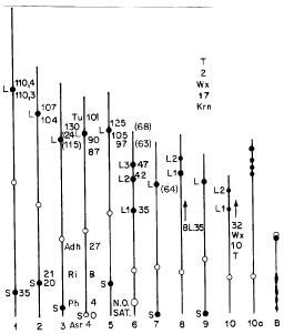
Kato (Mass. Agric. Exp. Stn. Bull. 635, 1976), concluded that the basic teosinte chromosome morphology has no knobs. He also observed that in the presence of inversions like in 4S and 9S involving knob sites, the knobs were absent. Kato and Lopes (Maydica 35:125-141, 1990) observed that in five sympatric populations of maize and teosinte, each pair had the same knob complex. McClintock (1978) presents an exhaustive discussion on knobs, together with a knob map from Kato, which we reproduce here. Figure 1 shows the distinctive components of the maize chromosome complement that were recorded in this study. From left to right the chromosomes are numbered according to the relative size, 1 to 10; 10a refers to Abnormal-10; B refers to the B-type chromosome. On the cytological map are superimposed the knob positions explained in the text of this report and also the new positions published in the MNL, 1992.

Classical biometrical models have been insufficient to solve the question. With the same Langham data, we developed a biometrical model for two pairs of alleles in the same chromosome affecting the same characters (tr and pd) in relation to a standard marker. This problem was already solved for a backcross case by Miranda et al. (MNL64, 1990). We propose now a model for F2 progenies.

With F2 progenies in repulsion, the gamete frequencies in relation to the marker gene are: pq, p(1-q), q(1-p) and (1-p)(1-q). Putting them in a 4x4 entry table, we obtain the genotypic expectations: p2q2, p2q(1-q) etc., until (1-p)2(1-q), (1-p)2(1-q)2 as in Table 2, where we see the genotypic expectations of classes, when two pairs of alleles affecting the same character (tr or pd) are calculated in relation to a marker within their span (repulsion phase):

Table 2.
 

Gametes	pq	p(1-q)	q(1-p)	(1-p)(1-q)
pq	p2q2	p2q(1-q)	pq2(1-p)	pq(1-p) (1-q)
p(1-q)	p2q(1-p)	p2(1-q)2	pq(1-q) (1-p)	p(1-p) (1-q)2
q(1-p)	pq2(1-p)	pq(1-p) (1-q)	q2(1-p)2	q(1-p)2 (1-q)
(1-p)(1-q)	pq(1-p) (1-q)	p(1-p) (1-q)2	q(1-p)2 (1-q)	(1-p)2 (1-q)2

The 16 genotypic classes or only 4 phenotypic classes can be identified as a, b, c and d, as usual. To class a corresponds the intersection of the 1st and 2nd lines with the 1st and 2nd columns; to b, the intersection of the 1st and 2nd lines with the 3rd and 4th columns and so on.

To class a the expectations are:

Factoring for p and adding we get

p² is the estimate for the a class. Effecting the same steps for b, c and d: p(1-p) is the b/n and c/n estimates and (1-p)² is the d/n estimate.

For the logarithmic likelihood expression, l being the normal log, and a, b, c and d the phenotypic classes observable we have:

Derivating in relation to p and adding we get

Putting the minimum common multiplier, factoring and equating to zero:

As we usually do, solving the quadratic equation we get the p value:

Making d²L/dp² to obtain the variance error we get:

Since V = -1/d²L/dp² the negative result offers a logical sense, following a Cramer-Rao inequality. This is the 11th theorem.

We can get an alternative simpler solution. If we first derivate the 16 classes and only after we pool them in classes a, b, c and d, we get:

The variance is obtained as usual:

being Vb = b(n-b)/n

The same is true for Vc and Vd. This is the 12th theorem.

For coupling, the formulae are:

or

Table 3 shows the analysis results of original data from Langham (Genetics 25:88-107, 1940). From the first column, chromo-;some number; genetic composition; values in cM of p calculated for a 9:3:3:1 inheritance, including the allometric effects alpha and beta; values in cM resulting from the analysis by the new model proposed in this report, for duplicated pairs of alleles in the same chromosome, as tr2 pd2 and tr12 pd12, affecting the same character; the standard errors; chromosome map distances (including markers used), obtained by the sum or differences in cM, intrapolating for chromosome 1 (pd2 and tr2) and for chromosomes 3 and 6. By difference, extrapolating for pd12 tr12 in chromosome 2 and in chromosomes 4 and 5. Note the overall strong linkage between pd's and tr's. The values in the 7th column were calculated with data from the 3rd column.

Table 3.
 

Chromosome	Genotype	cM (conventional)	cM (new model)	s	Genotype	cM (S differences)	s
1	fl pd	52	20.6	2.1	f1	86	0
	fl tr	85.2	22.8	2.1	tr11	110.3	1.5
	bm2 pd	128	23	2.1	pd11	110.4	1.5
	bm2 tr	49	25.7	2.4	bm2	161	0
2	lg1 pd	70	22.4	1.9	lg1	11	0
	lg1 tr	59.9	26.7	1.9	pd2	20	1.4
	gl2 pd	81.9	24.4	1.9	tr2	21	1.4
	gl2 tr	66.4	29.1	1.9	gl2	30	0
	b pd				v4	83	0
	b tr	71.1			pd12	104	1.9
					tr12	107	2.7
	v4 pd	86.3	20.7	1.9
	v4 tr	83	23.9	1.9
3	lg2 pd	36.5	21	2.5	lg2	101	0
	lg2 tr	59.3	25.1	2.5	tr3	124	1.7
	a1 pd	59.9	13.7	2.5	pd3	130	1.7
	a1 tr	58.2	27.9	2.5	a1	149	0
4	ts5 pd	56.1	32.6	2.7	ts5	53	0
	ts5 tr	45.6	50.4	3.3	su1	63	0
	su1 pd		27.5	3.4	pd14	87	3.4
	su1 tr		16	3.4	tr14	90	4.8
5	pr pd	99.2	30.1	3.1	.i.pr	67	0
	pr tr	58.2	38	3.1	pd15	97	3.1
					tr15	105	4.4
6	y1 pd		24.1	1.9	y1	17	0
	y1 tr	70.6	28.5	1.9	pd6	42	1.4
	py pd	54.9	26.6	1.9	tr6	47	1.2
	py tr	34.3	21.7	1.8	py	69	0

To check it, with Langham's data, lg pd, a = 160, b = 38, c = 50 and d = 9. Applying the models (I) and (III) we get the same result p = 0.2217899. As there is no available reference, we demonstrated the solutions in two ways, to cross-check it.

The results presented in Table 3 were calculated as follows:
    1. The distances to each marker were calculated for pd and tr.
    2. The p values were then converted to cM using Haldane's formula.
    3. The distances between pd and tr were obtained by differences of the cM values to the common marker.

For chromosome 1 the values obtained were interpolated within the fl bm2 distance as being pd11 at 103.4 and tr11 at 110.3, since probably there is a krn1 in position 35 as reported by Miranda et al. (MNL61, 1987).

For chromosome 2, interpolating within lg2 gl2 we get pd2 at 20 and tr2 at 22 since we had already an estimation of krn2 in position 22 (Miranda et al., MNL64, 1990). The values with v4 were used to get the sequence pd12 at 104 and tr12 at 107.

For chromosome 3, interpolating we get tr3 at 124 and pd3 at 130; this agrees with Miranda et al. (MNL61, 1987) and with K3L at 115 from Dempsey, E (1975).

For chromosome 4, extrapolating we get pd14 at 87 and tr14 at 90 because probably there is already a tr4 as suggested by Miranda et al. (MNL59, 1985). Miranda et al. (MNL63, 1989) proposed the sequence pd4 at 3, krn4 at 7 and ts5 at 53. The same authors, using the original Galinat, W's data (MNL49, 1975), measured ri su = 29, e and ph ri = 12. With su now in position 47 as a basis, this would lead to ph at 6 and ri at 15.

In chromosome 5 we get pd5 at 97 and tr5 at 105, probably the same as proposed by Miranda et al. (MNL61, 1987) as krn5 at 125.

In chromosome 6, interpolating we get tr6 at 42 and pd6 at 47, probably identical or one of a string reported by Miranda et al. (MNL61, 1987) as being in position 35. See the accompanying article putting K6L, with Dempsey's data, at position 41.

We can see that now the distance pd tr varies from 0.1 to 8.0 with a mean of 5, which demonstrates a much more biologically minded model.

In chromosome 7 krn7 at 64 is postulated by Miranda et al. (MNL61, 1987).

In chromosome 8, Miranda et al. (MNL58, 1984) reported results with translocations at 8L.09; 9S.16; 9S.31, studying flint characteristics in crosses with the Cateto line C2. Dent characteristic linkage was detected in individual grains as a dimple in the crown, as those exerted in baby cheeks in the act of smiling.
As shown in the same report, as krn, fas and flt are linked together, another pair, tr and pd, is demonstrated in a distal position to the latter marker.

In chromosome 9, the same authors found the sequence T - 2 - wx - 4 - flt9 - 13 - krn9 with the inversion at 9S.7; 9L.9. Nothing more can be inferred since there are knob sites in both arms of the chromosome.

In chromosome 10 the order and direction of T - 10 - wx - 32 - flt10 is given for a T at 9S.13; 10S.40 (Miranda et al., MNL61, 1987). The position is confirmed by the presence of knob sites only in the end of the long arm.

Of particular interest to this work is that from Kato (Evolut. Biol. 17:219-253, 1984). On knobs with restricted distribution he states:
    a) Mean Pacific Migration Path. This migration path is illustrated by the distribution pattern shown by the medium and large knobs in the short arm of chromosome 4. This knob appears to be concentrated in collections of the races Zapalote Chico and Zapalote Grande in Oaxaca-Chiapas.
    b) Northern Migration Path from Central Mexico. This migration path is exemplified by the distribution of the medium knob at the 6L1 position. The center of distribution of this knob is located in the Central Highlands of Mexico (Mesa Central) and is found in races such as Conico, Palomero Toluqueno, Arrocillo Amarillo and Chalqueno.
    c) Pepitilla Migration Path. This path is illustrated by the distribution of the large knob at the 6L3 position. It is characteristic of Pepitilla and Maiz Ancho.
    d) Mexican East Coast Migration Path. The specific knob that characterizes this migration path is the distribution of the large knob at the 9L2 position. It is characteristic of Tuxpeno.
    e) Migration Path from Highland Guatemala. The highland maize, typically represented by the races San Marceno, Serrano, Quicheno, Negro and Salpor, is characterized by the predominance of a combination of small knobbed and knobless positions. There is one specific small knob at the 10L1 position.
    f) Maize from South America is characterized by a typical knob distribution in chromosomes 6 and 7.
The author cites Galinat, who suggested that knobs may be linked to gene complexes controlling the essential taxonomic traits differentiating maize from teosinte. Beadle, GW (Maize Breeding and Genetics, ed. D. B. Walden, 1978) states that teosinte pops, and we remember that most primitive maize, including archaeological maizes, are popcorns.

In conclusion, the contention of Galinat (Adv. Agron. 47:203-231, 1992) that there is only one tr in chromosome 2 and only one pd in chromosome 3 seems untenable. Pego (Genetic Potential of Portuguese Maize with Abnormal Ear Shape, Ph.D. Thesis, Iowa State Univ., 1982) cites a report about P40, a fasciated popcorn inbred with 40 kernel rows in the ear. It seems reasonable that, since a tr pd pair accounts for 4 rows, there is a necessity of at least 10 pairs to achieve that row number.

Part of these conclusions are corroborated by Doebley, J (Trends Genet. 8:302-307, 1992). See also that in the recent chromosome 4 working map, published in the Maize Genetics Cooperation Newsletter (1992), the genetic cartography asr1 at 0; rp4 at 5; ri1 at 8; ga1 at 13; adh2 at 27 and su1 at 47 seems stimulating since it resembles the teosinte x maize affair. ga1 is just another way to flare the limits and asr1 and adh2 could find excellent biological reasons to be in the same neighbourhood.

Figure 1.

Return to the MNL 67 On-Line Index
Return to the Maize Newsletter Index
Return to the MaizeGDB Homepage