Confirmatory factor analysis of morphological variables of the ear and kernel in popcorn cultivars
--Burak, R, Broccoli, AM
In order to confirm the relationship between morphological variables of the ear and kernel of popcorn cultivars (Zea mays L.), experimental trials were developed in 1999, 2000 and 2001 in Esteban Echeverría and Luján (Buenos Aires, Argentina). These areas belong to a landscape called “Pampa Ondulada”, with hills that have the best soils for agriculture, classified as molisols, with 4.5 % organic matter.
Seventeen popcorn cultivars, commercial hybrids and native free pollination varieties, were planted, with a density of 70,000 plants/ha. Field trials were conducted under random complete blocks in a factorial arrangement: 17 treatments × 3 repetitions × 2 locations × 3 years. Experimental units were two rows of 5 m in length, with a distance between rows of 0.70 m.
Harvest maturity was reached at 135 days after sowing. Then kernels were homogenized at 14% moisture, and 306 measures of each variable were further developed.
The variables analyzed were:
Grain yield, kg/experimental unit (YIELD): this variable wsere measured by cutting grains of all kernels of each experimental unit and recording the weight of homogenized grains at 14 % moisture.
Expansion volume, gr/cc (EXVOL): volume of grains expanded in standard conditions (Dofing et al., 1990), obtained using a pop machine with temperature control by thermostat and temperature sensor under the plate. Expansion volume value was obtained by the relationship between the exploded sample volume measured in a test tube of 1,000 ml, and the volume of 30 cc of seed without exploding of the same sample, measured in a test tube of 150 ml.
Grain roundness index (GRI): the higher expansion volume usually attained from samples with medium to small kernels, rounder than the average, has been reported in classic papers, indicating the roundness index GRI, which is the relationship between thickness (KTH), width (KW) and length (KL) of the seed.
GRI = KTH / KW + KL
Harvest index (HI): calculated by the ratio No. of ears/No. of plants by experimental unit.
Percentage of cob (COB): calculated by the ratio weight of the kernels/weight of the ears.
Kernel volume in cubic centimeters (KXCC): Amount of grain in 1ml of volume.
Kernel per row (KFIL): mean of grain in the row of each experimental unit.
Longitude ear (EARL): measured in cm from the base to the apex of the ear.
Diameter ear (EARD): diameter in mm of the middle part of the ear.
To confirm the relationships among variables, factorial analysis by the principal component method was used, according to this model:
yij = μj + l1j × Fi1 + l2j × Fi2 + l3j × Fi3 + … + lmj × Fim + εij
yij = Value of the ith observation of the jth measured variable.
μj = Means of the jth variable.
Fik = Value of the ith observation on the kth common factor.
lkj = Regression coefficient of the kth common factor for predicting jth variable (loading factor).
εij = Value of the ith observation on the kth only factor.
m = Number of common factors.
Statistical analyses were run with SAS/STAT software (Version 8.1), the FACTOR PROCEDURE (See appendix SAS program). The initial factor method: principal component variance with N=3 factor shows that the explained variance by each factor is: factor 1 = 4.37, factor 2 = 1.22 and factor 3 = 0.896, with a total of 6.478285. Variance is retained by two first and second factors, therefore these are the only factors considered in analysis. Kaiser’s measure equaled 0.83245, which shows an optimal adaptation of the sample.
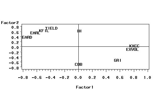
Commonalities are common variance estimations between variables and mean proportion of variance, with each variable contributing to the final solution. Commonalities less than 0.5 are considered as lacking sufficient explanation; as shown in Figure 1, with the exception of IH and COB, the rest of the variables are significantly contributing to the final solution.
The load factors matrix rotates; it is multiplied per one orthogonal matrix. Therefore, this allows a better interpretation of common factors, due to the simplification of the structure of these, and re-distributes variance since the former to the latter for achieving a simplest and, theoretically, a more significant pattern of factors. Table 1 shows rotated factors and non-rotating factors. Variances explained by each factor after rotation are similarly arranged (2.918 for factor 1 and 2.664 for factor 2).
Rotation by the varimax method (orthogonal transformation matrix) used in this work, gives a clearer separation of factors. Trends show that there are high factorial loads close to 1 or −1), and another near 0 in each column of the matrix. This means a clear association, negative or positive, between variable and factor; near zero involves an absence of association. To evaluate the contribution of each variable to the final solution, an empiric rule is applied. This suggests that factorial loads plus ± 0.3 represent a minimal level, ± 0.4 are important and ≥ ± 0.5 are considered significant. Table 1 shows rotated loads which each one of the variables develops on factors and common variance estimations among these variables (commonality). Variables KXCC, EXVOL and GRI make positive and significant loads on factor 1 (an unobserved variable that includes expansion capacity and its components), while EARL, EARD, YIELD, KFIL and IH develop positive loads on factor 2 (an unobserved variable that represents yield and components). Excepting IH, the rest of the variables associated with factor load negatively on factor 1, resulting in antagonism with factor 1 (Fig. 1). Also, variables IH and COB do not influence factor 1. IH loads positively on factor 2, while COB negatively. IH could be taken as a selection character for improving yield without affecting the expansion capacity of grain.
Table 1. Unrotated and rotated (Method varimax,. orthogonal transformation matrix) factor pattern, (N=2) and commonality estimates.
| Variables | Unrotated | Rotated (Method varimax) | Communality | ||
| Factor 1 | Factor 2 | Factor 1 | Factor 2 | ||
| KXCC | -0.557 | 0.598 | 0.815 | 0.062 | 0.668 |
| EXVOL | -0.625 | 0.480 | 0.788 | -0.067 | 0.626 |
| GRI | -0.758 | 0.022 | 0.573 | -0.498 | 0.576 |
| EARL | 0.851 | 0.013 | -0.616 | 0.586 | 0.724 |
| EARD | 0.820 | -0.190 | -0.733 | 0.417 | 0.716 |
| YIELD | 0.801 | 0.299 | -0.385 | 0.762 | 0.729 |
| KFIL | 0.809 | 0.158 | -0.488 | 0.665 | 0.681 |
| IH | 0.436 | 0.488 | 0.0102 | 0.655 | 0.429 |
| COB | -0.454 | -0.481 | 0.0081 | -0.662 | 0.438 |
| Variance explained by each factor | 4.368 | 1.214 | 2.918 | 2.664 | Total = 5.582 |
Figure 1. Plot of factor pattern for factor 1 and factor 2.
Appendix: SAS program.
|
DATA pop; TITLE 'popcorn'; INPUT YIELD KFIL EARL EARD EXVOL GRI COB KXCC IH; CARDS; 3.12 26 12.5 27 33.01 0.39 20.7 5.75 0.98 . . . . . . . . . . . . . . . . . . 3.63 35 16.2 31 15.31 0.25 19.9 4.16 0.91 run; PROC FACTOR DATA=pop res N=3; title 'method principal component unrotated' res N=3; VAR YIELD KFIL EARL EARD EXVOL GRI COB KXCC IH; run; PROC FACTOR DATA=pop res N=2 out=sal_pop outstat=estad; title 'method principal component unrotated' N=2; VAR YIELD KFIL EARL EARD EXVOL GRI COB KXCC IH; run; data estad; set estad; where _type_='PATTERN'; run; proc transpose data=estad out=trans1(rename=(_name_=variable)); run; data anotar1; set trans1; xsys='2'; ysys='2'; text=variable; x=factor1; y=factor2; run; symbol1 v=none; proc gplot data=trans1 anno=anotar1;title ' '; plot factor2*factor1=1/vref=0 href=0; run; symbol1 v=plus c=red; proc gplot data=sal_pop; title ' '; plot factor2*factor1=1; run; PROC FACTOR DATA=pop N=2 rotate=varimax preplot plot reorder round out=sal_pop outstat=estad; title 'metohd principal component' N=2; VAR YIELD KFIL EARL EARD EXVOL GRI COB KXCC IH; run; data estad; set estad; where _type_='PATTERN'; run; proc transpose data=estad out=trans1(rename=(_name_=variable)); run; data anotar1; set trans1; xsys='2'; ysys='2'; text=variable; x=factor1; y=factor2; run; symbol1 v=none; proc gplot data=trans1 anno=anotar1;title ' '; plot factor2*factor1=1/vref=0 href=0; run; symbol1 v=plus c=red; proc gplot data=sal_pop; title ' '; plot factor2*factor1=1; run; proc cluster data=sal_pop outtree=tree_pop method=single; var factor1 factor2; run; proc tree data=tree_pop; *out=out n=2; copy factor1 factor2; run; symbol1 v=circle c=black; symbol2 v=star c=black; symbol3 v=plus c=black; legend1 frame cframe=white cborder=black position=center value=(justify=center); axis1 minor=none label=angle=90 rotate=0=; axis2 minor=none; proc gplot; plot factor1*factor2=cluster/frame cframe=white vaxis=axis1 haxis=axis2 legend=legend1; *title 'analisys' *title2 'Single Linkage'; *title3 'cluster with data'; run; proc cluster data=sal outtree=tree method=ward; var factor1 factor2; run; proc tree out=out n=2; copy factor1 factor2; run; symbol1 v=circle c=black; symbol2 v=star c=black; symbol3 v=plus c=black; legend1 frame cframe=white cborder=black position=center value=(justify=center); axis1 minor=none label=(angle=90) rotate=0; axis2 minor=none; proc gplot; plot factor1*factor2=cluster/frame cframe=white vaxis=axis1 haxis=axis2 legend=legend1; *title 'analisys' *title2 'Single Linkage'; *title3 'cluster with data'; run; |